Learning
Bits

“nscancor” is an R package for canonical correlation analysis (CCA) under constraints. As the name implies, the nscancor function has the same interface as cancor from the “stats” package, but supports enforcing constraints on the canonical vectors, such as non-negativity and sparsity.

The implemented algorithm is based on iterated regression (Sigg et al., 2007), and generalized deflation (Mackey, 2009) adapted from PCA to CCA. By using readily available constrained regression algorithms, it becomes straightforward to enforce the appropriate constraints for each data domain. And by using generalized deflation, each subsequent tuple of canonical variables maximizes the additional correlation not explained by previous ones.

I hope to do a proper writeup at a later date, but for now, here is an explanation of how to use the package and a demonstration of its benefits.

Two Data Domains

One benefit of sparse CCA is that constraining the cardinality of the canonical vectors acts as a regularizer, which can improve the generalization performance of the algorithm, measured by the correlation achieved on test data.

Let’s demonstrate the effect on the nutrimouse data set from the “CCA” package, which contains paired gene expressions (120 variables) and fatty acid concentrations (21 variables) for 40 mice. We use glmnet in pure LASSO mode (alpha = 1) as the sparse regression function to predict the canonical variable yc associated with the fatty acid data Y from the gene expression data X:

1
2
3
4
5
6
7
8

ypredict <- function(X, yc, cc) {
  model <- glmnet(X, yc, alpha = 1, intercept = FALSE, 
                  dfmax = wcard + 10)
  W <- coef(model)
  idx <- max(which(cardinality(W) <= wcard), 2)
  w <- V[2:nrow(W), idx]
  return(w)
}

The desired cardinality of the canonical vector w associated with X is specified in wcard. Terminating glmnet using the cardinality stopping criterion dfmax works only in approximation, so we stop glmnet a little later and find the solution with the desired cardinality in line 5. The definition of xpredict is analogous and therefore not shown here.

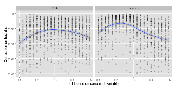
The correlation of the first pair of canonical variables is shown in the following figure. To make the presentation a bit more interesting, we compare nscancor to the CCA function from the “PMA” package (Witten, Tibshirani and Hastie, 2008), which implements a different approach to sparse CCA:

The scatter plots show fifty random splits into training and testing data (per sparsity bound), where a smaller bound corresponds to a sparser solution. The correlation achieved on test data is quite noisy because the number of samples in the nutrimouse data set is small. But as can be seen from the added smoother, there is an optimal cardinality for both algorithms.

Several Pairs of Canonical Variables

For the second pair of canonical variables, the CCA objective is again to maximize the correlation, but under the additional constraint that the second pair has to be uncorrelated to the first pair. For classical CCA, the solution involves an eigenvalue decomposition (EVD) of the covariance and cross-covariance matrices. The EVD provides all pairs of canonical vectors.

However, if constraints are enforced on the canonical vectors, they no longer correspond to eigenvectors. The constrained canonical vectors can be non-orthogonal, and variables of different pairs can have non-zero correlation. The CCA objective therefore has to be modified to obtain a well posed problem under constraints. The approach taken by generalised deflation is to maximize the additional correlation not explained by previous pairs of canonical variables. The acor function computes this measure.

Let’s demonstrate sparse CCA with several pairs of canonical variables, again on the nutrimouse data set. The prediction functions have to be modified slightly, such that different cardinalities can be specified for different canonical variables:

1
2
3
4
5
6
7
8

ypredict <- function(X, yc, cc) {
  model <- glmnet(X, yc, alpha = 1, intercept = FALSE, 
                  dfmax = wcard[cc] + 10)
  W <- coef(model)
  idx <- max(which(cardinality(W) <= wcard[cc]), 2)
  w <- W[2:nrow(W), idx]
  return(w)
}

cc is the counter for the current canonical variable, which makes it possible to specify the desired cardinalities of the canonical vectors associated with X in the array wcard.

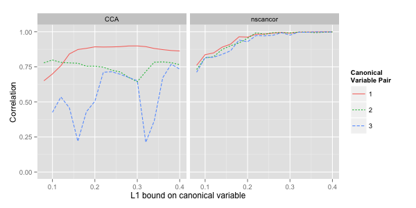
The following figure shows the correlations achieved on training data for the first three pairs of canonical variables. We should expect to see two effects:

1. The correlation curves should increase monotonically and ultimately approach unity, because the data sets contain more features than samples.

2. Less additional correlation is explained by subsequent pairs of canonical variables.

Both effects are present in the nscancor results (modulo some small random fluctuations). The results for CCA are inferior in two ways. Less correlation can be explained for the same sparsity bound, and the additional correlation explained by subsequent pairs of canonical variables is significantly lower. The erratic curve for the third pair of canonical variables suggests that the CCA algorithm can get stuck in poor local optima.

Multiple Data Domains

Classical CCA was formulated for pairs of correlated canonical variables. A generalization to three or more data domains should consider the full correlation matrix of the canonical variables. Therefore, the objective of multi-domain CCA can be defined as finding an \(m\)-tuple of canonical variables, such that the element-wise sum of its correlation matrix is maximal.

CCA for multiple data domains is implemented in the mcancor function. The functional nature of R makes it easy to generate the appropriate prediction function for each domain:

 1
 2
 3
 4
 5
 6
 7
 8
 9
10
11
12
13
14

generate_predfun <- function(card) {
  force(card)
  return(
    function(X, sc, cc) {
      model <- glmnet(X, sc, alpha = 1, intercept = FALSE, 
                      dfmax = card[cc] + 10)
      W <- coef(model)
      idx <- max(which(cardinality(W) <= card[cc]), 2)
      w <- W[2:nrow(W), idx]
      return(w)
    }
  )
}
predfuns <- lapply(cardinalities, generate_predfun)

cardinalities is a list of vectors, specifying the desired cardinality for each canonical vector of each domain. The call to force is necessary to avoid lazy evaluation of the card argument.

Let’s do a comparison of mcancor and MultiCCA, the equivalent function from the “PMA” package. The breastdata (also from the “PMA” package) contains 89 samples of gene expression and DNA copy number measurements. The data set for a three-way analysis of the RNA and the DNA from the first two chromosomes is constructed in the following way:

1
2
3
4
5
6
7
8

X <- with(
  breastdata, 
  list(
    scale(t(rna), TRUE, TRUE), 
    scale(t(dna)[ , chrom == 1], TRUE, TRUE), 
    scale(t(dna)[ , chrom == 2], TRUE, TRUE)
  )
)

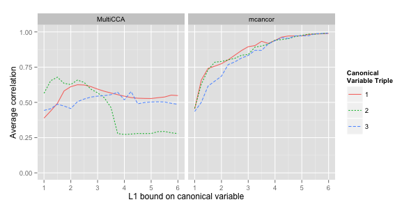
The following figure plots the average correlation between the canonical variables of the different domains, i.e. the average of all off-diagonal values of the correlation matrix. The correlation is again measured on training data, so we expect to see the same two effects as before:

And indeed the results are analogous. mcancor achieves both a better trade-off between explained correlation and sparsity of the canonical vectors, and explains more additional correlation in the second and third triple of canonical variables.

Conclusions

The three experiments did show that nscancor and mcancor achieve a good trade-off between sparsity and explained correlation, both for the first and subsequent tuples of canonical variables.

Other constraints, such as non-negativity, smoothness or structured sparsity of the canonical vectors can be enforced by plugging in the respective regression algorithm.

References

C. Sigg, B. Fischer, B. Ommer, V. Roth and J. Buhmann (2007). Non-Negative CCA for Audio-Visual Source Separation. Proceedings of the IEEE Workshop on Machine Learning for Signal Processing.

L. Mackey (2009). Deflation Methods for Sparse PCA. Advances in Neural Information Processing Systems.

D. Witten, R. Tibshirani and T. Hastie (2008). A Penalized Matrix Decomposition, with Applications to Sparse Principal Components and Canonical Correlation Analysis. Biostatistics 10(3), pp. 515-534.